The Deep Dive into Embedding Models: From Training to Advanced Techniques

Embeddings are the linchpin of modern AI, acting as the universal translator that converts complex, high-dimensional data like text, images, and audio into a language that machine learning models can understand: dense vectors of real numbers. These vectors capture the semantic essence of the data, allowing models to grasp relationships, similarities, and nuances.

But what exactly are these models? How do you build one from the ground up? And what are the cutting-edge techniques that push the boundaries of what's possible?

This deep dive will answer all these questions. We'll explore the different types of embedding models, walk through the process of training them from scratch, and unravel advanced techniques that make them more powerful and efficient.

The Spectrum of Embedding Models 🗺️

Embedding models can be broadly categorised based on the type of data they are designed to handle.

1. Text Embeddings

These models focus solely on natural language.

Static Embeddings: Models like Word2Vec and GloVe were pioneers. They generate a single, fixed vector for each word, capturing general semantic relationships (e.g., "king" - "man" + "woman" ≈ "queen"). However, they can't handle polysemy (words with multiple meanings, like "bank").
Contextual Embeddings: Modern transformer-based models like BERT, RoBERTa, and their sentence-level derivatives like Sentence-BERT (SBERT) generate embeddings that change based on the surrounding context. The word "bank" will have a different vector in "river bank" versus "investment bank." These are the standard for most NLP tasks today.

2. Multimodal Embeddings

These are the next frontier, designed to understand relationships between different types of data.

Image-Text Models: The most prominent example is CLIP (Contrastive Language-Image Pre-Training) from OpenAI. CLIP learns to map images and their corresponding textual descriptions to a shared "embedding space." In this space, the vector for a photo of a dog is positioned very close to the vector for the text "a photo of a dog." This enables powerful zero-shot image classification and image-text retrieval.
Other Modalities: The principles extend to other data types, with models being developed for video, audio, and text, allowing for a more holistic understanding of complex data.

From Scratch: A Guide to Training Embedding Models 🛠️

While pre-trained models are widely available, training your own embedding model on a specific domain can yield significant performance boosts. Here’s how it's done.

Training Text Embedding Models

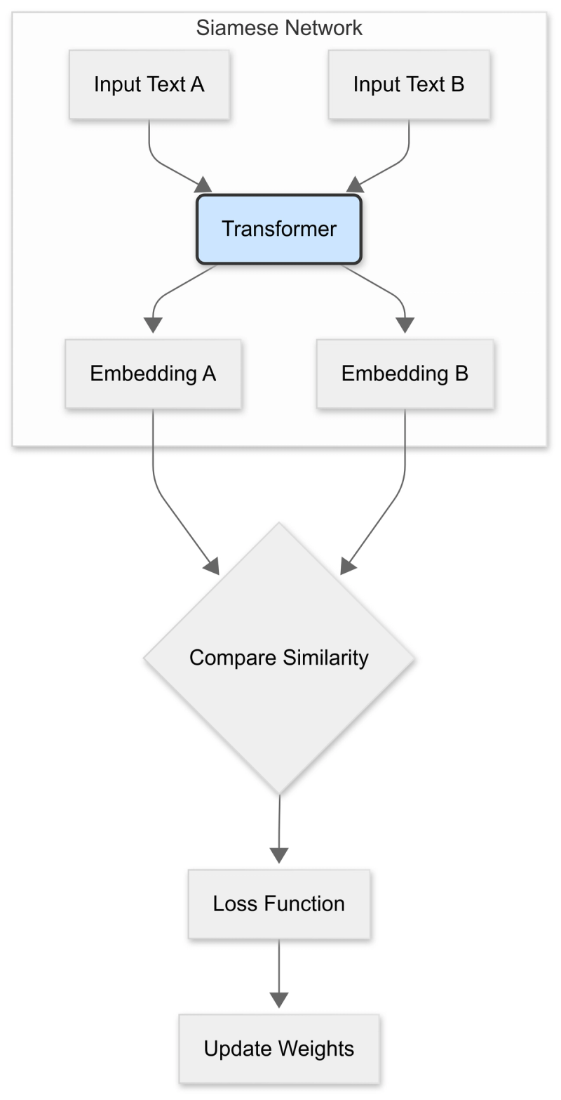
The goal is to teach the model what "similar" means. We do this by training a network, typically a Siamese or Triplet Network, to pull similar text pairs together in the vector space while pushing dissimilar ones apart.

Step 1: Data Preparation You need structured data that tells the model what is similar.

Pairs: For a Contrastive Loss approach, you need pairs of sentences labeled as either similar (positive pair, label 1) or dissimilar (negative pair, label 0).
- Positive Pair: ("The cat sat on the mat", "A feline was on the rug")
- Negative Pair: ("The cat sat on the mat", "I like to eat pizza")
Triplets: For a Triplet Loss approach, you create sets of three: an anchor, a positive (similar to the anchor), and a negative (dissimilar to the anchor).
- Triplet:
  - Anchor: "The weather is sunny today."
  - Positive: "It's a bright and sunny day."
  - Negative: "The car needs a new engine."

Step 2: Model Architecture The standard architecture uses a pre-trained transformer model (like BERT or RoBERTa) as the core encoder. In a Siamese Network, you pass two sentences through the same encoder (with shared weights) to get their respective embeddings. A pooling layer (often mean pooling) is added on top of the transformer's output to get a single fixed-size sentence vector.

Step 3: The Loss Function This is the magic that arranges the vector space.

Contrastive Loss: This function calculates the distance between the embeddings of a pair. For a positive pair, it tries to minimize this distance. For a negative pair, it tries to maximize the distance up to a certain margin.
Triplet Loss: This is often more effective. It aims to ensure that the distance between the anchor and the positive is smaller than the distance between the anchor and the negative by at least a predefined margin. The formula is: L=max(d(a,p)−d(a,n)+textmargin,0)
Multiple Negatives Ranking Loss: A highly efficient and popular method used by SBERT. Given a sentence (anchor) from a batch of size N, it treats its paired sentence as the positive and the other (N-1) sentences in the batch as negatives. It then uses a simple classification loss to identify the true positive, which is computationally much cheaper than forming explicit triplets.

Training Multimodal Embedding Models (e.g., CLIP)

The goal here is to align the vector spaces of two different modalities, like images and text.

Step 1: Data Preparation You need a massive dataset of (image, text) pairs. This is the biggest hurdle. The original CLIP was trained on a dataset of 400 million such pairs scraped from the internet. For a custom model, you'd curate a dataset relevant to your domain (e.g., product images and their descriptions).

Step 2: Model Architecture You use a dual-encoder architecture:

An Image Encoder (e.g., a Vision Transformer - ViT or ResNet) that takes an image and outputs an image embedding.
A Text Encoder (e.g., a Transformer like BERT) that takes a text caption and outputs a text embedding.

Both encoders are trained simultaneously to project their outputs into a shared, aligned embedding space.

Step 3: The Loss Function The training uses a symmetric contrastive loss. For a batch of N (image, text) pairs:

You get N image embeddings (I) and N text embeddings (T).

You compute the cosine similarity of every possible image-text combination, creating an NtimesN similarity matrix.

The goal is to maximize the similarity for the N correct pairs (found on the diagonal of the matrix) while minimizing the similarity for the N2−N incorrect pairs (off-diagonal).

The loss is calculated symmetrically: once by treating the images as queries against the text, and again by treating the text as queries against the images. This ensures robust alignment in both directions.

Tailoring Embeddings for Specific Tasks 🎯

Sometimes, a general-purpose semantic embedding isn't enough. Advanced models allow you to specify a task type to optimize the embeddings for a downstream application. This is not a simple flag; it reflects a change in the training or model architecture itself.

For retrieval (Asymmetric Search)

In retrieval tasks (e.g., semantic search), you often have a short query and a long document. These are not semantically identical, and a standard symmetric model might struggle. The solution is to use an asymmetric architecture:

You train two different transformer models: one for encoding queries and another for encoding documents.
The training objective remains the same (e.g., using Multiple Negatives Ranking Loss), but the model learns to map short queries to the region of the vector space that contains the relevant long documents. This is how models like msmarco-bert-base-dot-v5 are trained.

For classification or clustering

For these tasks, you need embeddings that form tight, well-separated clusters. While a general model can be used, fine-tuning it with a classification objective can improve performance.

How it's done: You add a "classification head" (a simple feed-forward neural network) on top of your embedding model.
Training: You train the entire system on a labeled dataset using a standard classification loss like Cross-Entropy Loss. This process not only trains the classification head but also fine-tunes the underlying embedding model, pushing the embeddings for the same class closer together and pulling embeddings for different classes apart.

Advanced Embedding Techniques 🚀

The field is constantly evolving. Here are some advanced techniques that address efficiency, performance, and memory usage.

1. Quantization

A standard float32 embedding takes up significant memory. Quantization reduces this footprint by converting the vectors to a lower-precision format.

Scalar Quantization: Converts float32 numbers to int8. This reduces memory usage by 4x and can speed up similarity calculations with a small-to-moderate loss in accuracy.
Binary Quantization: An extreme form where each dimension of the vector is reduced to a single bit (0 or 1). This offers a massive 32x reduction in size and allows for ultra-fast distance calculations using the Hamming distance. It's suitable for applications on resource-constrained devices, though it comes with a more significant accuracy trade-off.

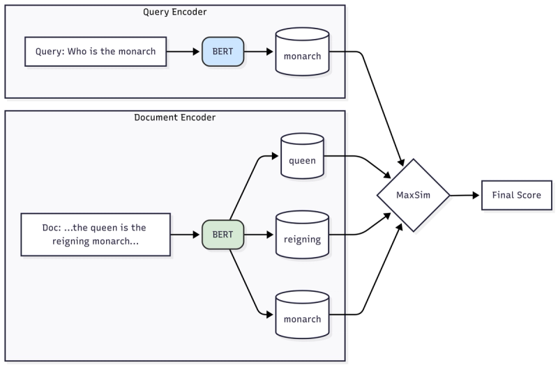
2. Late Interaction Models (e.g., ColBERT)

Traditional embedding models use a "late-stage" comparison: they convert an entire document into a single vector and then compare it with a query vector. This can lose fine-grained details.

ColBERT (Contextualized Late Interaction over BERT) offers a more nuanced approach:

Instead of one vector per document, it creates a vector for every token in the document.
At query time, it also generates a vector for every token in the query.
The relevance score is calculated by finding the maximum similarity for each query token against all document tokens and then summing these maximum scores. This "late interaction" allows for a much more precise matching of specific terms and phrases.

3. Matryoshka Representation Learning (MRL)

What if you didn't have to choose a fixed embedding dimension? MRL, inspired by Russian nesting dolls, trains embeddings so that prefixes of the full vector are themselves good, lower-dimensional embeddings.

A model trained with MRL might produce a 768-dimensional vector where:

The first 64 dimensions work well as a standalone small embedding.
The first 128 dimensions provide a better medium-sized embedding.
The full 768 dimensions give the best performance.

This is incredibly useful for applications that need to balance accuracy and computational cost dynamically. You can use the small embeddings for a fast initial search and then re-rank the top results using the larger, more accurate embeddings.

Conclusion

Embedding models are a foundational technology in AI, turning raw data into meaningful representations. From the contextual power of BERT to the cross-modal understanding of CLIP, they have unlocked incredible capabilities. By understanding how to train them from scratch, tailor them for specific tasks, and leverage advanced techniques like ColBERT and MRL, you can build more intelligent, efficient, and powerful AI systems. The journey into the vector space is just beginning.